Week 1 (Jan 15 - 17)
Read: Scaling in Art and Nature (ASGv2 Chap. 1).
Key topics: Dimensional analysis, units, scaling, review of algebra techniques.
PHY 201 lecture: Dimension analysis of the trinity nuclear test.
Key topics: Dimensional analysis, units, scaling, review of algebra techniques.
PHY 201 lecture: Dimension analysis of the trinity nuclear test.
Homework: Here are some homework problems involving the concepts of dimensional analysis and scaling. You may work on these with a friend, but you must write up and submit your own solutions. To receive full credit, your solutions must be handed in to me by noon on Tuesday of Week 2. These problems serve as practice to prepare you for quizzes and tests. Any homework submitted late will receive half credit.
Lab: Pendulum experiment. In this lab experiment we will practice keeping a lab notebook, careful measurement, experimental uncertainty, and dimensional analysis. You will need to bring your own laboratory notebook to class. Here is a nice place to buy them (external link). I have prepared some notes on propagating experimental uncertainty; these can be found here (pdf file).
Chapter 1 (4 videos): You should watch all of the videos. They are designed to lead you through Chapter 1 of A Student's Guide, in which Galileo begins his discussion dimensional analysis and scaling.
Additional lectures on Dimensional Analysis (2 videos): You should watch these; they will help you in solving the HW problems.
Perhaps of interest: For the biologists: here is a nice modern discussion of how living organisms' anatomy varies with their size. This approach is largely derived from Galileo's discussion of scaling in his Dialogues.
Trinity Atomic Bomb energy yield problem (PHY 201 students will work through this problem in class on Thursday and submit it as part of their homework)
On July 16, 1945, the United States Government tested the first atomic weapon in what is now the White Sands Missile Range in New Mexico. The energy released during the explosion was kept secret, but several photographs of the explosion were published in Life magazine. Some of these are shown below. Notice that the length scale and the time elapsed is indicated on each photograph.
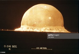
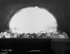
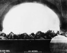
By analyzing photos like these, British physicist G.I.Taylor was able to correctly determine the energy released by this atomic explosion. How did he do it? By (i) observing how the blast radius increases as time elapses and (ii) using the technique of dimensional analysis.
Put the problem this way: the radius of the blast depends on the total energy released, E, the surrounding air density, d, and the time elapsed, t. That is: r = r (E, d, t). So what combination of E, d, and t will have the dimension of length? See if you can work it out. Hint: the blast radius does not increase linearly with time. But by plotting the blast radius versus the time—raised to some appropriate power, one can then determine the blast energy, E. In particular, the energy can be calculated using only the -slope- of the graph and the density of air (about 1.2 kg per cubic meter).
Here is data of the radius of the blast as a function of time:
t(msec), r (meters)
######, ########
0.10, 11.1
0.24, 19.9
0.38, 25.4
0.52, 28.8
0.66, 31.9
0.80, 34.2
0.94, 36.3
1.08, 38.9
1.22, 41.0
1.36, 42.8
1.50, 44.4
1.65, 46.0
1.79, 46.9
1.93, 48.7
3.26, 59.0
3.53, 61.1
3.80, 62.9
4.07, 64.3
4.34, 65.6
4.61, 67.3
15.0, 106.5
25.0, 130.0
34.0, 145.0
53.0, 175.0
62.0, 185.0
- Scaling of a sphere (Ex. 1.1)
- Kleiber's Law (Ex. 1.2).
- Dimensional analysis for the speed of a traveling wave: The speed of a wave traveling on the surface of the ocean depends only on (i) its wavelength and (ii) the acceleration of gravity. Using the technique of dimensional analysis, find a mathematical formula for the speed of the wave.
- Dimensional analysis for the frequency of a vibrating mass: find a mathematical formula for the frequency of vibration of a mass "m" attached to a spring with spring constant "k". You may need to look up the dimensions of the spring constant.
- PHY 201 students: Dimensional analysis for the trinity nuclear bomb test: Using dimensional analysis, make an appropriate plot of the data (given below). From the slope of your graph, determine the energy released by the first nuclear bomb test. Check to see how close you are to the published energy.
Lab: Pendulum experiment. In this lab experiment we will practice keeping a lab notebook, careful measurement, experimental uncertainty, and dimensional analysis. You will need to bring your own laboratory notebook to class. Here is a nice place to buy them (external link). I have prepared some notes on propagating experimental uncertainty; these can be found here (pdf file).
- Study the guidelines for how to keep a laboratory notebook.
- Suspend a pendulum bob from two thin cords so that it oscillates in a plane without rotating. You may use a ring stand, string, and a horizontal clamping bar.
- Pull your pendulum back, release it, and measure the time for one oscillation. For precision, you might wish to film your pendulum or repeat your measurements (or both).
- Record the following information in your notebook: How far did you pull your pendulum bob back before releasing it? How long was the string? What is the length of the pendulum? What is the weight of the pendulum bob? Be sure to estimate and record the uncertainty in each of your measured quantities.
- Repeat this procedure for several different cord lengths, recording your procedure and data in your lab book notebook
- Using Logger Pro, make a (beautiful) plot of the period of oscillation as a function of the pendulum length. Be sure to clearly label your axes and make your data points large and visible (but not too large). If your plot is not very good, you should collect some more data until you are confident that you have good results.
- Does your data behave as you expect, based on dimensional analysis? Fit an appropriate mathematical function to your data to see if it matches your expectations. This will involve using Logger Pro's curve fitting menu. You can use the help menu to assist you if necessary (or ask your instructor).
- Print your plot and fix it into your laboratory notebook. Your plot axes should be clearly labelled and your data should take up the entire area of your graph. In other words: make your plot look big and beautiful.
- Explain what you learned from your experiment and what you would do differently if you were to do the experiment again.
- Scan and submit all of the laboratory notebook pages from our pendulum experiment this week via the Canvas course management system. Your lab notebook pages must be submitted as a single file. Each page must be clearly readable. If I cannot read your writing and see your data points in your graphs, then I cannot grade your work.
Chapter 1 (4 videos): You should watch all of the videos. They are designed to lead you through Chapter 1 of A Student's Guide, in which Galileo begins his discussion dimensional analysis and scaling.
Additional lectures on Dimensional Analysis (2 videos): You should watch these; they will help you in solving the HW problems.
Perhaps of interest: For the biologists: here is a nice modern discussion of how living organisms' anatomy varies with their size. This approach is largely derived from Galileo's discussion of scaling in his Dialogues.
Trinity Atomic Bomb energy yield problem (PHY 201 students will work through this problem in class on Thursday and submit it as part of their homework)
On July 16, 1945, the United States Government tested the first atomic weapon in what is now the White Sands Missile Range in New Mexico. The energy released during the explosion was kept secret, but several photographs of the explosion were published in Life magazine. Some of these are shown below. Notice that the length scale and the time elapsed is indicated on each photograph.
By analyzing photos like these, British physicist G.I.Taylor was able to correctly determine the energy released by this atomic explosion. How did he do it? By (i) observing how the blast radius increases as time elapses and (ii) using the technique of dimensional analysis.
Put the problem this way: the radius of the blast depends on the total energy released, E, the surrounding air density, d, and the time elapsed, t. That is: r = r (E, d, t). So what combination of E, d, and t will have the dimension of length? See if you can work it out. Hint: the blast radius does not increase linearly with time. But by plotting the blast radius versus the time—raised to some appropriate power, one can then determine the blast energy, E. In particular, the energy can be calculated using only the -slope- of the graph and the density of air (about 1.2 kg per cubic meter).
Here is data of the radius of the blast as a function of time:
t(msec), r (meters)
######, ########
0.10, 11.1
0.24, 19.9
0.38, 25.4
0.52, 28.8
0.66, 31.9
0.80, 34.2
0.94, 36.3
1.08, 38.9
1.22, 41.0
1.36, 42.8
1.50, 44.4
1.65, 46.0
1.79, 46.9
1.93, 48.7
3.26, 59.0
3.53, 61.1
3.80, 62.9
4.07, 64.3
4.34, 65.6
4.61, 67.3
15.0, 106.5
25.0, 130.0
34.0, 145.0
53.0, 175.0
62.0, 185.0